You may also like...
Kobe's Legendary Jordans Command Half-Million at Auction

A player-exclusive pair of Air Jordan IIIs, worn and signed by Kobe Bryant during his 2002-03 'sneaker free agency' seas...
76ers Stun Celtics in Epic 3-1 Playoff Comeback

The Philadelphia 76ers achieved a historic Game 7 victory over the Boston Celtics, ending a 44-year playoff series droug...
Farewell to a Legend: 'Goodfellas' and 'Halloween' Actor Beau Starr Passes Away at 81

American actor Beau Starr, renowned for his roles as Sheriff Ben Meeker in the "Halloween" franchise and as Henry Hill's...
Hollywood Rejoices: SAG-AFTRA Strikes Tentative Deal on Studio Contract

SAG-AFTRA has reached a tentative four-year deal with major studios, successfully preventing new strikes and mirroring a...
ARIA Hall of Fame Celebrates 40 Years with New 2026 Inductees

The Australian Recording Industry Association has unveiled the six artists joining the 2026 ARIA Hall of Fame, celebrati...
Rivals Stars Bella Maclean & Alex Hassell Reveal Truth Behind Controversial Age-Gap Romance
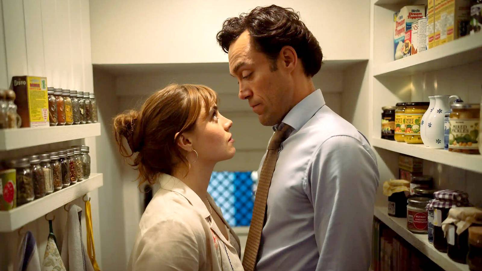
Hulu's 'Rivals' returns for its second season on May 15, promising an expanded cast, the introduction of polo, and deepe...
Nigeria: NDC Woos Obi, Kwankwaso Amid INEC Deadline Fault

The Nigeria Democratic Congress (NDC) has called on Peter Obi and Rabiu Kwankwaso to join its platform for the 2027 pres...
South Africa: Anti-Immigrant March Disrupts Pretoria

Over 300 individuals protested in Pretoria against undocumented immigrants and unemployment, led by March and March, wit...